|
return
to homepage
return
to updates
The
Proof for the Current Derivative
for Powers is False
by
Miles Mathis
Yes, I will
show that the proof of y' = nxn-1
is false. [To be clear, I am not
saying the equation is false, only the proof.] Not only
unnecessary, but false. I will re-prove it by a simpler and more
transparent method.
Many readers
don't understand why I would attack the calculus, so I try to
begin all these papers by reminding them that physics has hit
several major walls in the past century. Pure mathematicians may
not be aware of that, so they may not be aware that we have
empirical evidence that their maths are failing. I get emails
telling me that the calculus is the greatest thing ever invented
and that I am either an ingrate or a monster for looking closely
at it. But I am looking closely at it for a reason. The two
pillars of 20th century physics, Quantum Mechanics and General
Relativity, both hit similar walls. Many people know that they
have failed to be unified, but most people don't know that both
have to be renormalized. Renormalization is a big part of QED, as
is admitted, and GR also requires a sort of renormalization, a
push that is hidden in the tensor calculus and in the field
definitions. Renormalization was perfected by a famous physicist
named Richard Feynman, and he is notorious for calling his own
creation “hocus-pocus” that was “not
mathematically legitimate.” He also called it a shell-game.
What does renormalization do? It removes zeroes and infinities
from equations that are imploding or exploding. Why are these
equations imploding and exploding? No one knows. Richard Feynman
was the top mathematical physicist of his time, and Edward Witten
is the top mathematical physicist now. Witten has posed just this
question at Claymath, as one of the Millennium prizes. He wants
to know why the point maths of QED and QCD are failing. I have no
intention of submitting for this prize, since I know they will
not like my answer. But my answer is that the maths are failing
because they are based on the calculus, and that the calculus is
failing in QED because it is based on the point and on a move to
zero. This has also affected the search for unification, since
the mainstream is trying to unify by quantizing gravity. But
since they have misdefined the photon and other particles as
point particles, based on a misunderstanding of the calculus,
this effort is wasted.
Therefore, my work on the calculus
is neither capricious nor insolent. It may seem to overreach at
times, but it is always focused. It is focused on re-defining the
derivative and on jettisoning the point from all equations.
The
next complaint I hear is that I seem to have an aversion for
limits and infinities. In fact, I
don't1.
I believe some problems are best solved with limits: I just don't
think the calculus is one of them. The calculus can be solved by
simple number relations, because that is what creates the
equalities. As it turns out, proving the calculus with limits is
not only unnecessary and inefficient, it is false. It breaks
rules and finds fake numbers. It also warps fields and allows for
particles and motions that cannot exist. The problems embedded in
the calculus are what have caused many of the physical problems
in the past century.
Currently, modern mathematicians use
the calculus to find a derivative and a slope of the tangent by
taking Δx to zero. I
have shown2
many reasons they can't do that (and don't need to do that), but
the main reason is the one I will concentrate on in this paper:
it changes the given curve. If you go below 1 for the change of
your independent variable, you will have changed the curve. This
is important, because unless you also monitor that change, you
will get the wrong answer for your curve at x. I will show you
what I mean straight from the tables for x2
and x3.
Let Δx=1 (x= 1, 2, 3, 4...)
x2
= 1, 4, 9, 16, 25, 36, 49, 64, 81
x3
= 1, 8, 27, 64, 125, 216, 343
Δx2
= 3, 5, 7, 9, 11, 13, 15, 17, 19
Δx3
= 7, 19, 37, 61, 91, 127
ΔΔx2
= 2, 2, 2, 2, 2, 2, 2, 2, 2, 2
ΔΔx3
= 6, 12, 18, 24, 30, 36, 42
ΔΔΔx3
= 6, 6, 6, 6, 6, 6, 6, 6
Let Δx=.5
(x=.5, 1, 1.5, 2...)
x2
= .25, 1, 2.25, 4, 6.25, 9
x3
= .125, 1, 3.375, 8, 15.63
Let Δx=.25
(x=.25, .5, .75, 1...)
x2
= .0625, .25, .5625, 1, 1.5625
x3
= .01563, .125, .4219, 1, 1.95
If Δx=.5, then y =
x2
no longer has its original rate of change or curvature, as you
see. It has exactly ¼ the curvature it originally had. The
curve y = x3
loses much of its original curvature, too: it retains only 1/8 of
its curvature. If we continue taking Δx toward zero, by
making Δx=.25, this outcome is magnified. y = x2
has 1/16 of its curvature, and y = x3
has 1/64 of its curvature.
This shouldn't be happening,
and is not usually known to happen. You will not see the curves
analyzed in this way.
A critic will say, “Of course
the curve is straightening out. That is the whole point. We are
going to zero to magnify the curve. When you magnify a curve, its
loses its curvature at a given rate, depending upon the
magnification. Your curve x2
at Δx=.5 IS the same curve, it is just four times smaller.
”
True, but the curve should lose its curve at the
same rate you magnify it. If all the calculus were doing is
magnifying the curve, then if you magnified 2 times, the curve
would lose half its curve. If you are approaching zero in a
defined and rigorous manner, your magnification and curvature
should change together. But here, you magnify by 2 by halving
your Δx, but your curvature has shrunk to ¼ with x2
and to 1/8 with x3.
That is not a quibble, that is a major problem. If you change
your curve, you change your tangent.
My will critic will
answer, “It doesn't matter how much the curve changes as we
go in. We are going into a point, and the tangent only hits at a
point. Therefore the curvature won't change at that point.”
Wow, that sounds like pettifogging to me. By that
argument you can make the slope anything you want to at any point
on any curve. If changing the curvature doesn't really change the
curvature, then curvature has no meaning.
Currently, the
calculus just ignores this problem, or dodges it with oily
answers like that last one. To approach a limit in this way while
your given curve is changing would require a very tight proof to
convince me it is legal, and I have never seen one. If you dig,
you find that it requires an infinite line of proofs to “prove”
the legality of the first move to zero. For example, if you go to
Wikipedia, you will see the first in this line of proofs. Wiki
starts by telling us that the difference quotient
has
the intuitive interpretation that the tangent line to ƒ at a
gives the best linear approximation to ƒ near a (i.e., for
small h). This interpretation is the easiest to generalize to
other settings.
But
to tighten this up a bit, they next let the slope of the secant
Q(h) go to zero, and tell us
If
the limit exists, meaning that there is a way of choosing a value
for Q(0) which makes the graph of Q a continuous function, then
the function ƒ is differentiable at the point a, and its
derivative at a equals Q(0).
They still have
not proved anything there, they have just juggled some terms.
Notice they say, “IF the limit exists.” In fact, they
admit in the next sentence that the quotient is undefined at h=0,
which means the limit they have just created does not exist. You
cannot choose the value h=0, so their function is nullified.
Some will say that is an unnecessarily harsh judgment,
but it is no more than the truth. Every point on every curve
becomes a limit with the modern calculus, since whenever you
approach a value of x, you are approaching a limit to find the
derivative at that point. Q(0) exists not at the limit of some
given curve, it exists at every
point on that curve. Any point you desire to find a derivative
for becomes your limit of zero. So a curve is just a compendium
of limits. A curve becomes a sum of zeroes. Zeno
knew1
that was a paradox 2500 years ago, but the modern calculus still
boldly embraces it.
Wiki admits that taking Δx
(their h) to zero is a problem:
The
last expression shows that the difference quotient equals 6 + h
when h is not zero and is undefined when h is zero. (Remember
that because of the definition of the difference quotient, the
difference quotient is never defined when h is zero.) However,
there is a natural way of filling in a value for the difference
quotient at zero, namely 6. Hence the slope of the graph of the
squaring function at the point (3, 9) is 6, and so its derivative
at x = 3 is ƒ '(3) = 6.
More generally, a similar
computation shows that the derivative of the squaring function at
x = a is ƒ '(a) = 2a.
Do you see what
they just said? After 300 hundred years, this is the rigor we
get. Wiki tells us there is “a natural way of filling in a
value for the difference quotient at zero.” That just means
that we already know what the derivative is by looking at
differentials. We know the answer, so we push the difference
quotient to match it. That is the “natural way” of
solving this.
True, there are other more complex methods
for proving the move to zero. In fact, there are three centuries
worth of proofs, in hundreds of thousands of pages, from Newton
and Leibniz and Euler and Lagrange and Cauchy and Riemann so on,
all different and all in different notations. But if the answer
were clear, don't you think it could have been presented a bit
more quickly and easily than that? One would think that if the
move to zero were legal, it could have been shown immediately. In
my experience, only things that aren't
true require proofs of a million pages over many centuries.
I
think that just from what I have said, it is clear that the move
to zero is illegal. You cannot go to a limit to analyze a curve
when your curve is changing at a different rate than your
approach to the limit.
To solve, modern mathematicians
simply shrink Δx to suit themselves, never noticing or
caring that it must change the curve of the given curve. In other
words, they take a graph like the one below, draw the forward and
backward slopes (or secants, as the case may be), then begin
making them smaller and closer to their chosen point. Because it
all looks perfectly legal on the graph, no one ever questions the
legality of it. But I have just shown it is strictly illegal. If
you go below Δx=1, you will change your curve. If you have
made your Δx twice as small and at the same time your curve
is 4 times smaller, then your absolute curvature has changed.
There is no way around it.
But even if one or all of the
millions of pages of proofs are correct, it doesn't matter. Why
should we choose to solve this problem with a million pages of
difficult proofs, when we can solve it by looking at a few tables
of simple differentials? Why do teachers and textbooks and Wiki
reference all these complex proofs and never show us the simple
tables?
Regardless of the status of all these proofs,
going to zero wasn't necessary to begin with. We can find
specific slopes as well as general slope equations by several
other methods, and none of them use limits. We don't need to go
below Δx=1, because the forward slopes and backward slopes
will give us the slope at x by a simple average. Since x is
changing at a constant rate on the graph, the forward slopes and
backward slopes are the same size differentials, by definition.
The constancy of change in x assures us that our given value of x
is at the midpoint between forward and backward slopes. Just look
at the graphs: the change in x is always the same.
My
critic will say, “What you say is true of squared
acceleration, but you clearly don't understand cubed
acceleration. You can't find distances from cubed accelerations
by averaging, since the distance in the second period is much
greater than the distance in the first.” Well, that is also
true of squared acceleration. With a squared acceleration, the
distance in the second period is much greater than the distance
in the first. So that isn't the reason we can't (at first) seem
to average. The reason we can't seem to average with powers above
2 is that the power 2 changes at a constant rate of 2, but higher
powers don't.
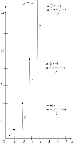 
Let
me show you exactly what I mean. We can find a slope for x2
very simply and accurately by averaging forward and backward
slopes, as you see from this graph. However, another similar
graph tells us we cannot get the current value of the slope that
way for x3.
Why? It is because the curve x2
is changing 3, 5, 7, 9. You can get that either from the table or
the graph. It is changing 2 each time. The curve x2
has a fundamental acceleration of 2. Therefore we can average in
one step. The average of 5 and 7 is 6, which is the slope at x=3.
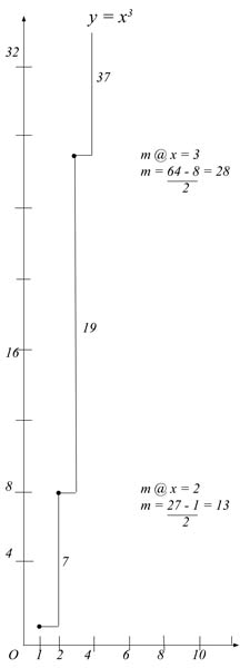
But the curve x3
is changing 7, 19, 37. It appears we can't average.
The
modern calculus tells us this is why we have to go to zero. We
can't average forward and backward slopes with most functions,
therefore we have to solve by going to zero. But that is false.
With x3
we don't have to go to zero any more than we did with x2.
We can find a derivative with a simple average. Like this.
Since x3
is changing 7, 19, 37, it has a fundamental acceleration of 6n
(where n=1, 2, 3). You can see that in the last two lines in the
table above. That being the case, our acceleration could be
written as this series:
1, 1 + 6, 1 + 12, 1 + 18, 1 +
36...
That is where the numbers 1, 7, 19, 37 come from.
So, if we want to find the slope at 3, say, that will be between
the numbers 19 and 37. Just consult the graph. I have shown that
we cannot average 19 and 37 directly, because that would give us
the number 28, which is not the current slope. But since the
curve is is achieved by a 1+ series, we can subtract the one away
from each term. If we do that, then our forward and backward
slopes at x=3 will be 18 and 36, in which case we can find the
current slope by averaging. (18 + 36)/2 = 27. That is the current
slope at 3. So we could
find a slope just by averaging, even with an acceleration of 6n.
You will say, “Wait, you just changed your curve by
doing that. You just proved that changing the curve was
forbidden, then you did it. You subtracted 1 away from your
series, and you now have this series:
Δx3
= 6, 18, 36, 60, 90
Those are the rates of change for 0,
6, 24, 60, 120, 210, not x3
= 1, 8, 27, 64, 125, 216.”
True, but the curve 0,
6, 24, 60, 120, 210 is still an acceleration of 6n, therefore it
is an acceleration above x2,
therefore you CAN find an average acceleration for powers above
2. You can't find it just by adding two numbers and dividing by
2, but you can find it. In this case, it is the forward slope
minus 1 plus the backward slope minus 1, over 2. It is still an
average, it is still very simple, and it doesn't require using a
limit.
m@(x,y) = {[Δy@(x+1)]
– 1} + {[Δy@(x)] – 1}
2
The same analysis applies to x4:
m@(x,y) = {[Δy@(x+1)]
– 12} + {[Δy@(x)] – 12}
2
Because we can average forward and backward slopes like
this with a general equation, it means the process is not an
accident or push.
Δx5
= 1, 31, 211, 781, 2101, 4651, 9031
m@(x,y) = {[Δy@(x+1)]
– (10x2 + 1)} + {[Δy@(x)] – (10x2 +
1)}
2
We can average powers above 2 because they are
constant. They are constant not as the power 2 is constant: the
power 2 is constant at the first rate of change. But all simple
powers are constant in that they increase in a consistent manner,
by a process that can be broken down. We can see that right from
the tables. If we take enough changes of any power, we see that
it is constant at a fundamental level. That is what 6, 6, 6, 6 is
telling us about x3.
Two rates down, it is constant. Therefore it is constant. That
was my point in a recent paper on “variable”
acceleration. Cubed acceleration is not really variable. It is
constant. It can be averaged, if you do it in the right way. It
is a consistent increase, therefore it can be analyzed in a
straightforward manner, as we are doing here. We don't need
limits, we can just use simple number relations.
Although
I have shown we can average forward and backward slopes with all
powers, the slope equations get very complicated as we advance
into the higher powers. We also encounter a problem with finding
slopes for values of x near 1, since we are subtracting large
numbers from our Δy's. This means we need a better way to
generalize our slope equation. I have already shown how to do
that in my long paper on the derivative. I will gloss it again
here.
We will pull the general equation straight from the
tables. We will start with the smaller powers. Since x3
is changing 7, 19, 37, it has a fundamental acceleration of 6n
(where n=1, 2, 3). You can see that in the last two lines in the
table above. Since x2
has a fundamental acceleration of 2, the fundamental acceleration
of x3
is 3 times that of x2
over each interval. Six is three times two. We can write that as
f
x3
= 3x2,
where f
means fundamental acceleration.
If we are physicists, or
logical people of any stripe, that proof of the derivative of x3
is much preferable to the current one. We don't go to zero, we
don't talk of limits or functions or infinitesimals or any of
that. We pull the general derivative equation straight from a
table of differentials, and in doing so we see right where all
the numbers are coming from. Now we just need to generalize that
equation. We can do that by analyzing other powers. By studying
the simple tables2,
we find that all other powers obey the same relationship we just
found between x2
and x3.
f
xn
= nxn-1
The
differentials themselves give us the derivative equation for
powers. This means we don't need any other proof of it. A table
of differentials is all the proof we need. It is a proof by “show
me.” You want me to prove that a dog is white, so I show
you the white dog. You want me to prove that the derivative
equation for powers is f
xn
= nxn-1,
so I show you the tables, with the numbers sitting right next to
each other. If you require a proof beyond that, we must call you
a confused and meddlesome person, and we recommend you go into
set theory, where you can write thousand-page books proving
tautologies (while ignoring much greater real problems sitting on
your desk).
I will answer one more question here before I
move on to the other more important questions on my
desk. A close reader will ask, “We can write the series 0,
6, 24, 60, 120, 210... as x3
– x, and you have shown that both the curve x3
– x and the curve x3
can be written as accelerations of 6n. By your abbreviated and
direct proof, both curves should have a derivative of 3x2.
But they don't. The derivative of x3
– x is 3x2
– 1. How do you explain that?”
Once again, I
am not here to show that the current derivatives for powers are
wrong. I am here to show that the proofs are wrong. I admit the
derivatives are different for x3
– x and x3,
but that difference can be shown and generalized without using
limits. In this case, the difference is caused by the first term
in the series. The first term in one series is 1 different from
the other, and so is the derivative. So the difference in
equations can be shown by simple demonstration, or by pointing to
a table. It doesn't require limits or difficult proofs. I have
not exhausted all the demonstrations, or answered all questions.
I am only here to suggest that every question has a simpler
answer than the one we have so far been shown, one that can be
achieved without limits. All calculus questions can be answered
by studying the tables, since the tables supply the actual number
relations that generate the calculus. Fundamentally, calculus is
about these number relations, not about limits or approaches to
zero.
Because the calculus is not about limits and can be
proved without limits, it cannot find solutions at points or
instants. My method differs from the modern calculus not only in
its simplified proofs, but in its definitions. Because Δx
is always 1 and cannot go below one, our derivatives and
solutions are always found over a defined interval of 1.
Instantaneous velocities and accelerations are impossible, as are
point particles and all other solutions at points. This solves
many of the problems of QED and General Relativity. It solves
renormalization directly, since the equations are never allowed
to become abnormal to begin with. And it disallows "mass
points" in the field equations. If you cannot have math at a
point, you cannot have mass at a point. Modern physicists have
been fooled by the calculus into thinking they can or should be
able to do things they simply cannot do. My correction to the
calculus disabuses them of this mistaken notion. They have had
problems with points in their math and their fields because
points do not exist, in either math or fields. Only intervals
exist. Only intervals can be studied mathematically. This is why
they call it the differential calculus. It is a calculus of
differentials, and differentials are always intervals. Just check
the epsilon/delta proof. It is defined by differentials, not
points. Mathematicians at all levels and in all centuries always
seem to forget that whenever it is convenient.
1http://milesmathis.com/zeno.html
2http://milesmathis.com/are.html
If this paper was useful to you in
any way, please consider donating a dollar (or more) to the SAVE
THE ARTISTS FOUNDATION. This will allow me to continue writing
these "unpublishable" things. Don't be confused by
paying Melisa Smith--that is just one of my many noms de
plume. If you are a Paypal user, there is no fee; so it might
be worth your while to become one. Otherwise they will rob us 33
cents for each transaction.
|